Heatmap 2SFCA

The Heatmap 2SFCA (Two-Step Floating Catchment Area) tool produces a color-coded map visualizing spatial accessibility by combining supply capacity and demand in a single measure.

1. Explanation

The 2SFCA method measures spatial accessibility by considering both supply (capacity of facilities) and demand (population). Unlike simple supply-demand ratios per administrative unit, 2SFCA accounts for cross-boundary access — people can reach facilities in neighboring areas, and facilities serve populations beyond their own district. The result is a supply-to-demand ratio at the level of hexagonal grid cells. The tool works in two steps:

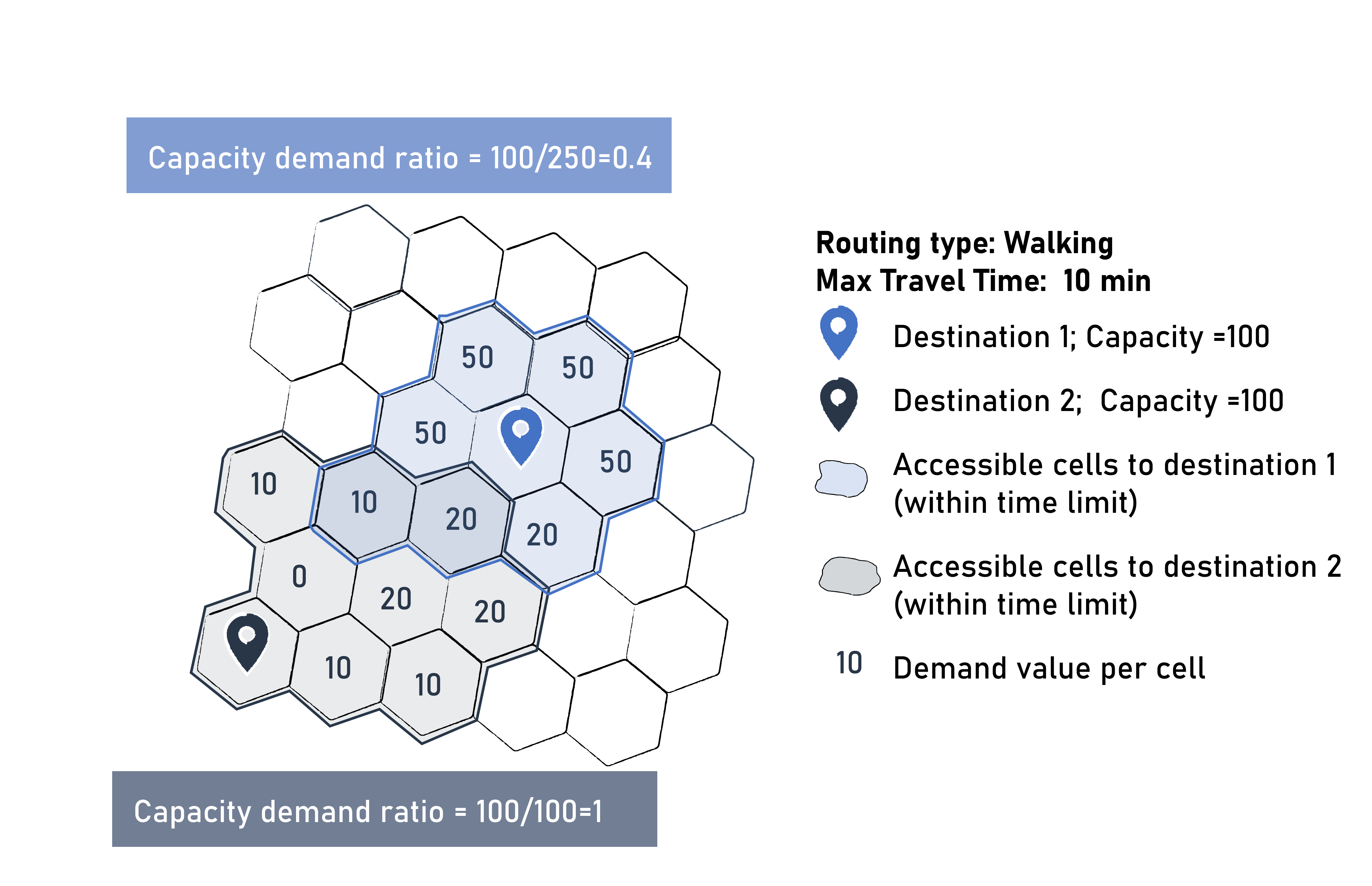
1. Step 1 — Capacity Demand Ratios: For each facility location, compute how much capacity is available relative to the total demand (population) within its catchment area. This produces a supply-to-demand ratio per facility.

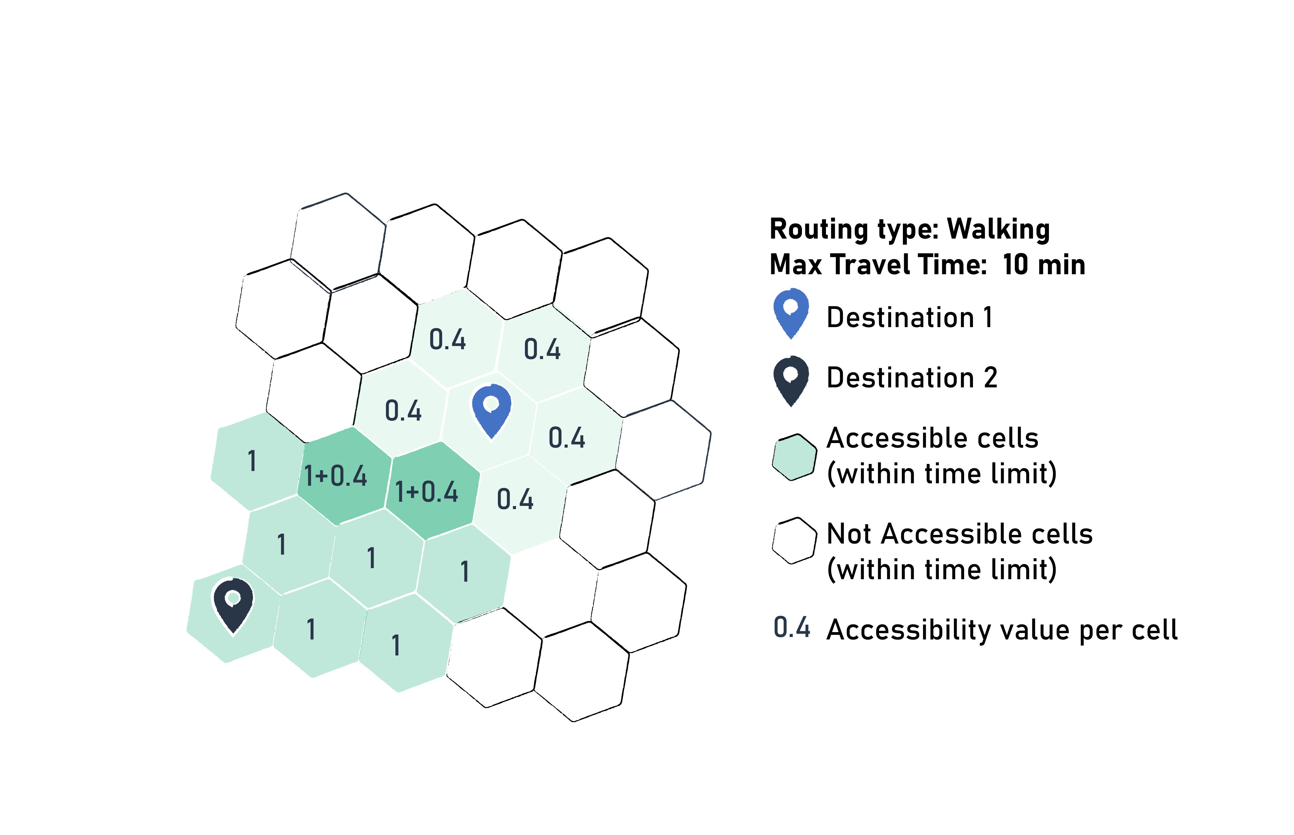
2. Step 2 — Cumulative Accessibility: For each grid cell, sum the capacity ratios of all reachable facilities. The result represents how well-served each location is.

You can configure the routing type, opportunity layers (with capacity fields), demand layer (with population field), travel time limits, and choose between three 2SFCA variants.

• The Opportunity layers contain facility data with a capacity attribute (e.g., number of hospital beds, square meters of retail space, school seats).

• The Demand layer contains population or user data (e.g., number of residents, potential customers) that represents the demand for the facilities.

• The 2SFCA Type controls how distance weighting is applied:

  • Standard 2SFCA uses binary catchments (in or out) - all locations within the travel time limit are weighted equally, regardless of their actual distance from facilities. This provides clear, straightforward supply-demand ratios.
  • Enhanced 2SFCA (E2SFCA) weights by an impedance function in both calculation steps, creating realistic distance decay where closer facilities contribute more to accessibility than distant ones.
  • Modified 2SFCA (M2SFCA) uses squared impedance weights in the second step, creating even stronger proximity bias. This variant heavily emphasizes nearby facilities while still considering distant options, making it ideal when travel convenience is paramount.

Key difference: Unlike the Gravity-based Heatmap, which measures general accessibility of destinations, the 2SFCA Heatmap explicitly models supply-demand balance — showing where capacity is sufficient or insufficient relative to the population that needs it.

info

Heatmaps are available in certain regions. Upon selecting a Routing type, a geofence will be displayed on the map to highlight supported regions.

Coverage for 2SFCA Heatmaps

If you would like to perform analyses beyond this geofence, feel free to contact us. We would be happy to discuss further options.

2. Example use cases

• Which neighborhoods are underserved by childcare facilities relative to the population that needs them?

• Where should new childcare centers be built to best address gaps in supply-demand balance?

• Are there areas where school capacity is insufficient given the number of school-aged children in the catchment?

3. How to use the tool?

1

Click on Toolbox .

2

Under the Accessibility Indicators menu, click on Heatmap 2SFCA.

Routing

3

Pick the Routing Type you would like to use for the heatmap.

Walk

Considers all paths accessible by foot. For heatmaps, a walking speed of 5 km/h is assumed.

Bicycle

Considers all paths accessible by bicycle. This routing mode takes into account the surface, smoothness and slope of streets while computing accessibility. For heatmaps, a cycling speed of 15 km/h is assumed.

Pedelec

Considers all paths accessible by pedelec. This routing mode takes into account the surface and smoothness of streets while computing accessibility. For heatmaps, a pedelec speed of 23 km/h is assumed.

Car

Considers all paths accessible by car. This routing mode takes into account speed limits and one-way access restrictions while computing accessibility.

Configuration

4

Select the 2SFCA Type you would like to use.

Standard 2SFCA

The standard 2SFCA method uses binary catchments: a facility either serves a population location (if within the travel time limit) or it does not. There is no distance weighting — all locations within the catchment are treated equally.

This is the simplest variant and works well when you want a straightforward supply-demand ratio.

Enhanced 2SFCA (E2SFCA)

The Enhanced 2SFCA method adds distance decay weighting using an impedance function. In both steps, interactions are weighted by how far apart the facility and population are — closer locations receive higher weight. This produces more realistic results, reflecting that people are more likely to use nearby facilities.

Requires selecting an impedance function and sensitivity value.

Modified 2SFCA (M2SFCA)

The Modified 2SFCA method applies squared impedance weights, creating an even stronger distance decay effect. While Enhanced 2SFCA considers proximity with a relative weighting approach, Modified 2SFCA also takes into account the absolute distance impact by squaring the impedance weights.

Requires selecting an impedance function and sensitivity value.

5

If using E2SFCA or M2SFCA, select the Impedance Function for distance weighting.

Gaussian

Calculates distance weights using a Gaussian (bell-shaped) curve. Accessibility decreases slowly for short travel times and drops off rapidly beyond a certain threshold. This is the most commonly used impedance function. For details, see Technical details.

Linear

Maintains a direct linear relationship between travel time and weight. Weight decreases uniformly from 1 (at origin) to 0 (at maximum travel time). For details, see Technical details.

Exponential

Calculates weights using an exponential decay curve, controlled by the sensitivity parameter. Higher sensitivity values produce a slower decay. For details, see Technical details.

Power

Calculates weights using a power function. The sensitivity parameter controls the exponent, determining how quickly weights decrease with travel time. For details, see Technical details.

Demand

6

Select your Demand Layer from the drop-down menu. This layer should contain population or user data (e.g., census data with resident counts).

7

Choose the Demand Field — a numeric field from your demand layer representing the number of potential users (e.g., population, number of households).

Opportunities

8

Select your Opportunity Layer from the drop-down menu. This layer should contain facility locations (e.g., hospitals, schools, shops).

9

Choose the Capacity Field — a numeric field representing the supply capacity of each facility (e.g., number of beds, seats, or square meters).

10

Set the Travel Time Limit defining the maximum catchment area in minutes.

Hint

Need help choosing a suitable travel time limit for various common amenities? The "Standort-Werkzeug" of the City of Chemnitz can provide helpful guidance.

11

If using E2SFCA or M2SFCA, specify a Sensitivity value to control how quickly the impedance function decays with distance.

12

Optionally, add more opportunity layers by clicking + Add Opportunity. Multiple facility types can be combined into a single analysis.

13

Click Run to start the calculation.

Results

Once the calculation is complete, a result layer will be added to the map. This Heatmap 2SFCA layer contains a color-coded hexagonal grid where each cell shows the computed accessibility value — the supply-to-demand ratio at that location.

• Higher values indicate better accessibility: more supply capacity is available relative to the local demand.
• Lower values indicate underserved areas: the population exceeds the available capacity of reachable facilities.

Clicking on any hexagonal cell reveals its computed accessibility value.

Tip

Want to create visually compelling maps that tell a clear story? Learn how to customize colors, legends, and styling in our Styling section.

Example of calculation

The following example illustrates how the 2SFCA method works for each step.

• Step 1 computes a capacity ratio for each destination. A destination with 100 beds serving 100 people has a ratio of 1.

• Step 2 sums up the ratios of all destinations reachable from each cell. A cell that can reach two destinations (ratios 1 and 0.4) gets an accessibility of 1.4.

4. Technical details

Calculation

The 2SFCA method computes accessibility in two steps:

Step 1 — Capacity Demand Ratio

For each facility location j, compute the ratio of its capacity to the total demand within its catchment:

Where:

• R_j = capacity demand ratio of facility j
• S_j = capacity (supply) of facility j
• D_k = demand (population) at location k
• d_kj = travel time from location k to facility j
• d₀ = travel time limit (maximum catchment)
• f(d_kj) = impedance function (distance weight)

Step 2 — Cumulative Accessibility

For each grid cell i, sum the capacity demand ratios of all reachable facilities:

Where:

• A_i = accessibility at location i
• R_j = capacity demand ratio of facility j (from Step 1)
• f(d_ij) = impedance function weight

2SFCA Variants

The three variants differ in how the impedance function f(d) is applied:

Variant	Step 1	Step 2
Standard 2SFCA	f(d) = 1 (binary)	f(d) = 1 (binary)
E2SFCA	f(d) = w(d)	f(d) = w(d)
M2SFCA	f(d) = w(d)	f(d) = w(d)2

Where w(d) is the selected impedance function (Gaussian, Linear, Exponential, or Power).

Comparison of variants

The different calculation approaches change how distance is perceived and measured, as illustrated in the examples below. Each scenario shows a facility with 100 units of capacity (indicated by the central location marker) serving grid cells with 50 units of demand each. We assume a maximum travel time of 5 minutes, where small arrows represent 1-minute travel time and large arrows represent 2-minute travel time. A linear impedance function ($f(d) = 1 - d/5$) is used for Enhanced and Modified variants.

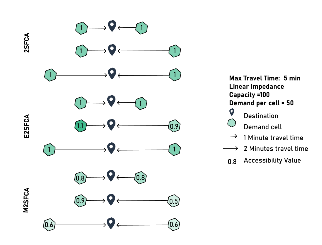
• The Standard 2SFCA treats all locations within the catchment equally, regardless of distance. Whether a population cell is 1 minute or 2 minutes away from the facility, it receives the same value in all configurations of 1.

• The Enhanced 2SFCA introduces distance decay weighting producing differenciation of the accessibility based on the distance, with a higher accessibility (value of 1.1) for closer cells. However, cells equidistant from facilities receive identical accessibility regardless of absolute distance (e.g., two cells both 1-minute away or in 2-minute away all get 1).

• The Modified 2SFCA applies squared impedance weights in Step 2, producing stronger distance penalties with values like 0.9 and 0.5 (compared to E2SFCA's 1.1 and 0.9 for similar positions). It takes into account absolute distance in opposition to E2SFCA — for example, two cells both 2 minutes away get lower accessibility (0.6) than two cells both 1 minute away (0.8).

Choosing the appropriate variant depends on your specific analysis objectives and how sensitive your target population is to travel distance.

GOAT uses the following impedance functions for the Enhanced and Modified 2SFCA variants:

Modified Gaussian, (Kwan,1998):

Pro tip

As studies have shown, the relationship between travel time and accessibility is often non-linear. This means that people may be willing to travel a short distance to reach an amenity, but as the distance increases, their willingness to travel rapidly decreases (often disproportionately).

Leveraging the sensitivity you define, the Gaussian function allows you to model this aspect of real-world behaviour more accurately.

Cumulative Opportunities Linear, (Kwan,1998):

Negative Exponential, (Kwan,1998):

Inverse Power, (Kwan,1998) (power in GOAT):

Classification

In order to classify the accessibility levels that were computed for each grid cell, a classification based on quantiles is used by default. However, various other classification methods may be used instead. Read more in the Data Classification Methods section of the Attribute-based Styling page.

Visualization

Heatmaps in GOAT utilize Uber's H3 grid-based solution for efficient computation and easy-to-understand visualization. Behind the scenes, a pre-computed travel time matrix for each routing type utilizes this solution and is queried and further processed in real-time to compute accessibility and produce a final heatmap.

The resolution and dimensions of the hexagonal grid used depend on the selected routing type:

Walk

Resolution: 10

Average hexagon area: 11285.6 m²

Average hexagon edge length: 65.9 m

Bicycle

Resolution: 9

Average hexagon area: 78999.4 m²

Average hexagon edge length: 174.4 m

Pedelec

Resolution: 9

Average hexagon area: 78999.4 m²

Average hexagon edge length: 174.4 m

Car

Resolution: 8

Average hexagon area: 552995.7 m²

Average hexagon edge length: 461.4 m

Hint

For further insights into the Routing algorithm, visit Routing. In addition, you can check this Publication.

5. References

Jörg, R.; Lenz, N.; Wetz, S.; Widmer, M. (2019): Ein Modell zur Analyse der Versorgungsdichte: Herleitung eines Index zur räumlichen Zugänglichkeit mithilfe von GIS und Fallstudie zur ambulanten Grundversorgung in der Schweiz (Obsan Bericht, Nr. 01/2019). Neuchâtel: Schweizerisches Gesundheitsobservatorium.

https://www.obsan.admin.ch/sites/default/files/obsan_01_2019_bericht_0.pdf