Huff Model
The Huff Model predicts the probability of consumers in a reference area visiting particular locations based on the attractiveness of the locations and the distance to those locations, including competition between opportunities. The Huff Model focuses on competitive market share.
1. Explanation
The Huff Model is a spatial interaction model that estimates how demand (e.g., customers, residents) is distributed among competing supply locations (e.g., stores, facilities). The model works on a simple principle: a location's probability of being chosen depends on its attractiveness relative to all competing locations, weighted by travel time. A large, nearby shopping center will capture more demand than a small, distant one — but the exact split depends on the balance of attractiveness and distance for all available options.
The result is a probability score for each supply location, representing the share of total demand it captures from the reference area. This enables direct comparison of how well different facilities compete for the same customer base.
You can configure the routing type, opportunity layers (with capacity fields), demand layer (with population field), reference area, travel time limits, and calibrate your model.
Reference area — A polygon defining the study area. Only demand and opportunities within this area are considered.
The Opportunity layers contain facility data with an attractivity attribute (e.g., number of hospital beds, square meters of retail space, school seats).
The Demand layer contains population or user data (e.g., number of residents, potential customers) that represents the demand for the facilities.
Key difference: Unlike the Heatmaps, which visualize accessibility per grid cell, the Huff Model produces a probability per supply location — showing what share of total demand each facility captures.
The Huff Model is available in certain regions. Upon selecting a Routing type, GOAT displays a map overlay showing the supported coverage area. If you need analyses beyond these regions, feel free to contact us.
2. Example use cases
How much market share does each supermarket capture from surrounding residential areas?
Where should a new retail store be opened to maximize customer reach while considering existing competitors?
How would adding a new school affect enrollment distribution across existing schools?
What share of demand does each public library capture from surrounding neighborhoods?
3. How to use the tool?
Toolbox  .
. Accessibility Indicators menu, click on Huff Model.Routing
Transport mode you would like to use for the analysis.| Mode | Considers | Speed assumed |
|---|---|---|
| Walk | All paths accessible by foot | 5 km/h |
| Bicycle | All paths accessible by bicycle (surface, smoothness, slope) | 15 km/h |
| Pedelec | All paths accessible by pedelec (surface, smoothness) | 23 km/h |
| Car | All paths accessible by car (speed limits, one-way restrictions) | — |
Configuration
Reference Area — a polygon layer defining the study area boundary. Only demand and opportunities within this area are included in the analysis.Travel Time Limit defining the maximum travel time in minutes. Facilities beyond this limit are not considered.Need help choosing a suitable travel time limit for various common amenities? The "Standort-Werkzeug" of the City of Chemnitz can provide helpful guidance.
Demand
Demand Layer from the drop-down menu. This layer should contain population or consumer data (e.g., census data with resident counts, customer locations).Demand Field — a numeric field from your demand layer representing the number of potential consumers (e.g., population, number of households).Opportunities
Opportunity Layer from the drop-down menu. This layer should contain facility or store locations that compete for demand.Attractivity Field — a numeric field representing the attractiveness of each facility (e.g., floor area in m², number of products, quality score).Advanced Configuration
Attractiveness Parameter (default: 1.0) to control how strongly attractiveness influences the probability. Higher values amplify differences between facilities.Distance Decay parameter (default: 2.0) to control how strongly travel time reduces a facility's appeal. Higher values mean people are less willing to travel far.For realistic results, the Huff Model parameters should be calibrated using observed market share or user choice data. The default parameters may not reflect actual customer behavior in your study area. Ideally, collect data on actual customer visits or market shares to estimate optimal parameters.
Note: Automated parameter calibration is not currently available in GOAT. You can manually adjust the parameters.
Result Layer
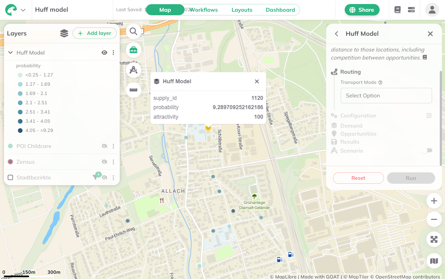
Result layer name for the output Huff Model layer.Run to start the calculation.Results
Once the calculation is complete, a result layer will be added to the map. Each feature in the result layer represents a supply location with its computed market share/probability expressed in percent.
- Higher probability values indicate that a facility captures a larger share of the total demand — it is more competitive relative to alternatives.
- Lower probability values indicate that a facility captures less demand, either because it is less attractive, farther away, or faces strong competition from nearby alternatives.
Want to create visually compelling maps that tell a clear story? Learn how to customize colors, legends, and styling in our Styling section.
4. Technical details
Calculation
The Huff Model computes the probability that demand from location i flows to supply location j:
Where:
- Pij = probability that demand at location i visits supply location j
- Aj = attractiveness of supply location j
- dij = travel time from demand location i to supply location j
- α = attractiveness parameter (default: 1.0)
- β = distance decay parameter (default: 2.0)
- n = number of supply locations reachable from i
The captured demand for each supply location is then computed by multiplying the probability by the demand value at each origin and summing across all origins:
Where:
- Cj = total captured demand at supply location j
- Di = demand (population) at location i
- m = number of demand locations
The final Huff probability reported per supply location is the share of total demand it captures:
5. References
Huff, D. L. (1963). A Probabilistic Analysis of Shopping Center Trade Areas. Land Economics, 39(1), 81–90.