Spatial Clustering

The Spatial Clustering tool creates clustered zones by grouping nearby features into a specified number of spatial clusters.

1. Explanation

The Spatial Clustering tool groups a set of spatial features into a specified number of spatial zones. It offers two clustering methods:

• K-Means — A fast, geometry-based method that groups features by proximity to cluster centers. This method does not aim to provide equal-sized zones.

• Balanced Zones — A genetic algorithm that creates zones with near-equal sizes, either by feature count or by a numeric field value. This method also supports compactness constraints to limit the spatial spread of each zone.

info

The Spatial Clustering tool is currently limited to point features only. It only supports a maximum of 2,000 points. For larger datasets, consider pre-filtering or sampling your data before running the tool.

info

• The Balanced Zones method uses a genetic algorithm which is non-deterministic. Different runs may produce slightly different zone configurations.
• Execution time for Balanced Zones can vary significantly based on the number of points and desired clusters. It is generally slower than K-Means, taking anywhere from 1 Minute to 3 minutes depending on dataset complexity.

2. Example use cases

• Dividing sales territories into balanced zones based on customer locations and revenue.

• Grouping population locations into areas with equal population size.

• Grouping potential car-sharing stations into service areas.

3. How to use the tool?

1

Click on Toolbox .

2

Under the Geoanalysis menu, click on Spatial Clustering.

Input

3

Select your Input Layer from the drop-down menu. This must be a point layer containing the features you want to cluster.

4

Set the Number of Clusters — the number of zones to create (default: 10).

Configuration

5

Select the Cluster Type.

K-Means

K-Means groups features by proximity to cluster centers. It is fast and suitable when you need a quick spatial grouping without strict size balancing.

No additional configuration is required for K-Means.

Balanced Zones

Balanced Zones uses a genetic algorithm to create zones with equal or near-equal sizes. This method is slower but produces more balanced results.

Additional configuration options become available:

6

If using Balanced Zones, select the Size Method: Count for equal features counts per zone, or Field Value to balance by a numeric attribute.

7

If using Field Value, select the Size Field — a numeric field from your input layer to use as the balancing weight.

8

Optionally, enable Limit Zone Area to add a compactness constraint. When enabled, configure the Max Distance to limit the maximum distance between two features in the same cluster.

9

Click Run to start the calculation.

Results

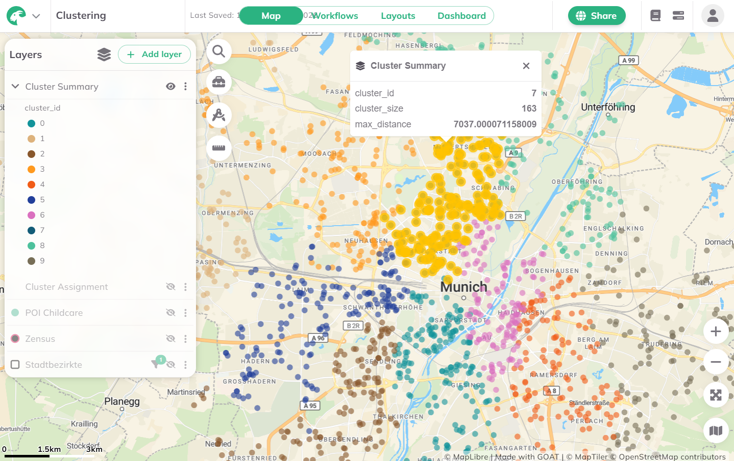
Once the calculation is complete, two result layers will be added to the map:

1. Features layer — The original input features, each assigned a cluster_id.
2. Summary layer — One multigeometry feature per zone, with zone statistics (size, maximum distance between features).

Tip

Want to create visually compelling maps that tell a clear story? Learn how to customize colors, legends, and styling in our Styling section.

4. Technical details

K-Means Clustering

The K-Means algorithm works iteratively:

1. Initialization — k initial centroids are chosen using a furthest-point strategy for better spread.
2. Assignment — Each feature is assigned to the nearest centroid based on Euclidean distance (in projected coordinates).
3. Update — Centroids are recalculated as the mean position of all assigned features.
4. Repeat until centroids converge or the maximum number of iterations is reached.

Balanced Zones

The Balanced Zones method uses a genetic algorithm to find optimal spatial groupings:

1. An initial population of solutions is created using K-Means as a starting point, plus random variations.
2. For each solution, extract seed for each cluster and grow zones through spatial neighbors to assign all features to clusters. Features unassigned by growth are assigned to the smallest surrounding cluster. The frontier features of large clusters can then be reassigned to smaller zones.
3. Each solution is scored based on a fitness score.
4. The best solutions are combined and mutated across multiple generations to progressively improve the result.
5. The algorithm stops when no further improvement is found or the maximum number of generations is reached.

The algorithm uses spatial neighbor graphs to ensure contiguous zone growth — features are assigned to zones through their spatial neighbors, promoting compact and connected clusters.

Fitness function:

Each candidate solution is scored based on:

• Size variance — How evenly the zones are sized (primary objective).
• Compactness penalty (optional) — Penalizes zones where the maximum distance threshold is exceeded.

All constraints (equal size, compactness) are soft constraints — the algorithm optimizes toward them but does not enforce them as hard limits.

Algorithm parameters:

Parameter	Value	Description
Population size	40–50	Number of candidate solutions per generation
Generations	40–50	Maximum number of evolutionary cycles
Mutation rate	0.1	Probability of changing cluster seed location
Crossover rate	0.7	Probability of combining parent solutions
Elitism	Top 10%	Best solutions preserved across generations

Adaptive parameters: For larger datasets (>500 features), the population size and generation count are automatically reduced to maintain reasonable computation times.